Basics of Oscilloscopes, Spectrum Analyzers, and Generators
Working with an oscilloscope...
It all starts with a dipstick !
The probe wire is coaxial. The central core of the probe is signal, braided ground (minus or common wire).
Some probes, especially modern oscilloscopes, have a voltage divider built inside (1:10 or 1:100) that allows you to measure a wide range of voltages. Before taking measurements, pay attention to the position of the toggle switch on the probe to avoid measurement errors.
The probe has a built-in compensation capacitor. In the low frequency band (below 300Hz) there is no effect on the gain, but in the 3kHz - 100MHz band a significant change in gain is obvious.
Oscilloscopes have an internal square wave generator, the signal of which is output to the front panel, to the “calibration” terminal. A calibration signal is provided specifically for adjusting the compensation capacity. The frequency of this signal is usually 1 kHz, with a swing of 1V. The probe is connected to the “calibration” terminal and adjusted to obtain the most correct signal shape.
We connect the probe to the oscilloscope...
The oscilloscope input can be closed or open . This allows the signal to be connected to amplifier Y either directly or through a coupling capacitor. If the input is open, then both DC and AC components will be supplied to amplifier Y. If private only variable. Example 1. We need to look at the ripple level of the power supply. Let's assume that the power supply voltage is 12 volts. The ripple value can be no more than 100 millivolts. Against the background of 12 volts, the ripples will be completely invisible. In this case we use a closed entrance. The capacitor filters out the DC voltage. Amplifier Y receives only an AC signal. Now the pulsations can be amplified and analyzed!
To scale the waveform on the screen, use the Gain and Duration .
The Gain knob scales the signal along the Y axis. It determines the cost of dividing one cell vertically in volts.
The Duration knob scales the signal along the X axis. It determines the cost of dividing one cell horizontally in seconds.
Example 2. Based on the values indicated by these knobs and the number of cells occupied by the signal, it is possible to determine the time parameters of the signal in seconds and its amplitude in volts. Based on these data, it is possible to calculate the pulse duration, pause, period and frequency of the signal.
In the case when the oscillogram does not fit on the screen and it is necessary to move it vertically or horizontally, use the vertical and horizontal movement handles .
To conveniently display cyclically repeating signals, synchronization . Synchronization ensures that individual pulses are drawn, always starting from the same point on the screen, thereby creating the effect of a still image.
The sweep mode determines the behavior of the oscilloscope. There are three modes: automatic (AUTO), standby (Normal), and single (Single).
Automatic mode allows you to capture images of the input signal even when trigger conditions are not met. The oscilloscope waits for the trigger conditions to be met for a certain period of time and, if the required trigger signal is absent, automatically starts recording.
Standby mode allows the oscilloscope to capture waveforms only when trigger conditions are met. If these conditions are not met, the oscilloscope waits for them to appear; the previous waveform is saved on the screen, if it was recorded.
In single acquisition mode , after pressing the RUN/STOP button, the oscilloscope will wait for the trigger conditions to be met. When they are executed, the oscilloscope will make a single acquisition and stop.
Trigger system determines the moment the oscilloscope begins to record data and display the waveform. If the trigger system is configured correctly, there will be clear oscillograms on the screen.
The oscilloscope supports a number of sweep trigger types : edge trigger, slope trigger, arbitrary edge trigger.
The trigger level is the voltage value at which the oscilloscope begins to draw the waveform.
Working with a spectrum analyzer...
There is a general technique for studying signals, which is based on decomposing signals into a Fourier series using an algorithm for quickly calculating the discrete Fourier transform, Fast Fourier Transform ( FFT ).
This technique is based on the fact that it is always possible to select a series of signals with such amplitudes, frequencies and initial phases, the algebraic sum of which at any time is equal to the value of the signal under study.
Thanks to this, it became possible to analyze the spectrum of signals in real time.
Let's look at the operating principle of a typical FFT analyzer .
The signal under study is received at its input. The analyzer selects successive intervals (“windows”) from the signal in which the spectrum will be calculated, and performs FFT in each window to obtain the amplitude spectrum.
The calculated spectrum is displayed as a graph of amplitude versus frequency.
FFT Length parameter , the length of the window - the number of analyzed signal samples - is crucial for the type of spectrum. The larger the FFT Length, the denser the frequency grid into which FFT decomposes the signal, and the more frequency details are visible on the spectrum.
To achieve higher frequency resolution, longer sections of the signal must be analyzed.
When it is necessary to analyze rapid changes in the signal, the window length is chosen to be small. In this case, the resolution of the analysis increases in time and decreases in frequency. Thus, the frequency resolution of the analysis is inversely proportional to the time resolution.
One of the simplest signals is a sinusoidal one. What will its spectrum look like on an FFT analyzer? It turns out that it depends on its frequency. FFT decomposes the signal not into the frequencies that are actually present in the signal, but into a fixed uniform frequency grid.
If the frequency of the tone matches one of the frequencies of the FFT grid, then the spectrum will look “ideal”: a single sharp peak will indicate the frequency and amplitude of the tone.
If the frequency of the tone does not match any of the frequencies in the FFT grid, then the FFT will “assemble” the tone from the frequencies available in the grid, combined with various weights. In this case, the spectrum graph is blurred in frequency. This blurring is usually undesirable because it can obscure weaker signals at adjacent frequencies.
To reduce the effect of spectrum blurring, the signal before calculating the FFT is multiplied by weighting windows - smooth functions falling towards the edges of the interval.
They reduce spectrum blur at the expense of some deterioration in frequency resolution.
The simplest window is rectangular : it is a constant 1 that does not change the signal. It is equivalent to the absence of a weight window.
One of the popular windows is the Hamming window . It reduces the smear level by approximately 40 dB relative to the main peak.
Weighting windows differ in two main parameters: the degree of broadening of the main peak and the degree of suppression of spectrum blur (“side lobes”). The more we want to suppress the side lobes, the wider the main peak will be. A rectangular window blurs the top of the peak the least, but has the highest side lobes.
The Kaiser window has a parameter that allows you to select the desired degree of sidelobe suppression.
Another popular choice is the Hahn window . It suppresses the maximum side lobe less than the Hamming window , but the remaining side lobes fall off faster with distance from the main peak.
The Blackman window has stronger sidelobe suppression than the Hahn window .
For most problems, it is not very important which type of weight window to use, the main thing is that it exists. Popular choices are Khan or Blackman . Using a weighting window reduces the dependence of the spectrum shape on a specific signal frequency and its coincidence with the FFT frequency grid.
To compensate for peak broadening when using weighting windows, longer FFT windows can be used: for example, 8192 samples rather than 4096 samples. This will improve the resolution of the analysis in frequency, but degrade it in time.
Working with a signal generator...
When it comes to measuring equipment, the first thing that comes to mind is, as a rule, an oscilloscope or logic analyzer ( recording instruments ).
However, these instruments can only perform measurements if they receive a signal.
There are many examples where such a signal is absent until an external signal is applied to the device under test.
Example. It is necessary to measure the characteristics of the circuit being developed and ensure that it meets the requirements.
Therefore, a set of instruments for measuring the characteristics of electronic circuits must include sources of the influencing signal and recording devices.
The signal generator is a source of the influencing signal.
Depending on the configuration, the generator can generate analog signals, digital sequences, modulated signals, intentional distortion, noise and much more.
The generator can create “ideal” signals or add specified distortions or errors of the desired magnitude and type to the signal.
Signals can take all sorts of forms:
- sinusoidal signals;
- square waves and square signals;
- triangular and sawtooth signals;
- drops and pulse signals;
- complex signals.
Signals of complex shapes include:
- signals with analog, digital, pulse-width and quadrature modulation;
- digital sequences and encoded digital signals;
- pseudo-random streams of bits and words.
One type of generator is a sweeping frequency generator. This is a special type of signal generator in which the frequency of the output signal changes smoothly over a certain interval and then quickly returns to the initial value. During this time, the amplitude of the output signal remains constant.
If a radio amateur has an oscilloscope at his disposal, then using it together with a sweep frequency generator, you can easily check and adjust quartz, electromechanical and LC filters, radio frequency and IF paths of the receiver or transmitter, and examine the frequency response of radio and television equipment in a wide frequency range.
The results of the comparison of technical characteristics and the internal structure of the measuring complex will be described in detail in the following video.
Tags:
- Digital oscilloscope
Blog about electronics
▌Old article about an analog oscilloscope
Sooner or later, any novice electronics engineer, if he does not give up his experiments, will grow up to circuits where it is necessary to monitor not just currents and voltages, but the operation of the circuit in dynamics. This is especially often needed in various generators and pulse devices. There is nothing to do here without an oscilloscope!
Scary device, right? A bunch of knobs, some buttons, and even a screen, and it’s not clear what’s there or why. No problem, we'll fix it now. Now I will tell you how to use an oscilloscope.
In fact, everything is simple here - an oscilloscope, roughly speaking, is just... a voltmeter! Only a cunning one, capable of showing a change in the shape of the measured voltage.
As always, I’ll explain with an abstract example. Imagine that you are standing in front of the railway, and an endless train consisting of completely identical cars is rushing past you at breakneck speed. If you just stand and look at them, you will see nothing but blurry garbage. Now we’ll put a wall with a window in front of you. And we begin to open the window only when the next carriage is in the same position as the previous one. Since our cars are all the same, you don’t necessarily need to see the same car. As a result, pictures of different but identical cars will pop up before your eyes in the same position, which means the picture will seem to stop. The main thing is to synchronize the opening of the window with the speed of the train, so that the position of the car does not change when opening. If the speed does not match, the cars will “move” either forward or backward at a speed depending on the degree of desynchronization.
A strobe is built on the same principle - a device that allows you to look at fast moving or rotating crap. There, too, the curtain opens and closes quickly.
So, an oscilloscope is the same strobe, only electronic. And it doesn’t show cars, but periodic voltage changes. For the same sinusoid, for example, each subsequent period is similar to the previous one, so why not “stop” it, showing one period at one time.
Design This is done by means of a beam tube, a deflection system and a scan generator. In the beam tube, a beam of electrons hitting the screen causes the phosphor to glow, and the plates of the deflection system allow this beam to be driven across the entire surface of the screen. The higher the voltage applied to the electrodes, the more the beam is deflected. By applying a sawtooth voltage to the X plates, we create a scan. That is, our beam moves from left to right, and then sharply returns and continues again. And we apply the voltage being studied to the Y plates.
Principle of operation Then everything is simple, if the beginning of the appearance of the saw period (the beam is in the extreme left position) and the beginning of the signal period coincide, then in one sweep pass one or more periods of the measured signal will be drawn and the picture will seem to stop. By changing the sweep speed, you can ensure that only one period remains on the screen - that is, during one period of the saw, one period of the measured signal will pass.
Oscilloscope time sweep
Synchronization You can synchronize the saw with the signal either manually, adjusting the speed with the handle so that the sine wave stops, or by level. That is, we indicate at what input voltage level we need to start the sweep generator. As soon as the input voltage exceeds the level, the sweep generator will immediately start and give us a pulse. As a result, the scan generator produces a saw only when necessary. In this case, synchronization is completely automatic. When choosing a level, you should take into account such a factor as interference. So if you take the level too low, then small needles of interference can start the generator when it is not needed, and if you take the level too high, then the signal can pass under it and nothing will happen. But here it’s easier to turn the knob yourself and everything will immediately become clear. The synchronization signal can also be supplied from an external source.
The theory is out of the way, let's move on to practice. I will show you the example of my oscilloscope, stolen a long time ago from the defense enterprise Design Bureau "Rotor" :). An ordinary oscil, not very sophisticated, but reliable and simple as a sledgehammer.
My trusty oscilloscope
So: I think the brightness, focus and illumination of the scale are self-explanatory. These are the interface settings.
Amplifier U and up and down arrows. This knob allows you to move the signal image up or down. Adding additional offset to it. For what? Yes, sometimes the screen size is not enough to accommodate the entire signal. We have to drive it down, taking the lower limit, rather than the middle, as zero.
Below is a toggle switch switching the input from direct to capacitive. This toggle switch in one form or another is found on all oscilloscopes without exception.
Important thing! Allows you to connect the signal to an amplifier either directly or through a capacitor. If you connect directly, then both the constant component and the variable will pass through. And only the variable passes through the condenser.
For example, we need to look at the noise level of the computer's power supply. The voltage there is 12 volts, and the amount of interference can be no more than 0.3 volts. Against the background of 12 volts, these measly 0.3 volts will be completely unnoticeable. You can, of course, increase the Y gain, but then the graph will go off the screen, and the Y shift will not be enough to see the top. Then we only need to turn on the capacitor and then those 12 volts of constant voltage will settle on it, and only the alternating signal will pass into the oscilloscope, those same 0.3 volts of interference. Which can be enhanced and seen in full height.
Next comes the coaxial connector for connecting the probe. Each probe contains a signal and ground. The ground is usually placed on the negative or on the common wire of the circuit, and the signal wire is poked according to the circuit. The oscilloscope shows the voltage on the probe relative to the common wire. To understand where the signal is and where the ground is, just grab them with your hand one by one. If you take the general one, then the corpse’s pulse will still be on the screen. And if you take up the signal signal, you will see a bunch of crap on the screen - interference to your body, which is currently serving as an antenna. Some probes, especially modern oscilloscopes, have a 1:10 or 1:100 voltage divider built inside, which allows you to plug the oscilloscope into an outlet without the risk of burning it. It turns on and off with a toggle switch on the probe.
Almost every oscilloscope also has a calibration output. On which you can always find a rectangular signal with a frequency of 1 KHz and a voltage of about half a volt. Depending on the oscillator model. Used to check the operation of the oscilloscope itself, and sometimes it comes in handy for testing purposes