Electrical equipment does not operate at full capacity all the time. This obvious fact can be understood using an everyday example. The lighting in the apartment is not turned on 24 hours a day. We use the iron only when we need to iron clothes. The kettle only works when you need to boil water. The situation is similar when it comes to electricity consumption in public and industrial buildings. Thus, the concept of installed and consumed (calculated) power is familiar to everyone since childhood. When designing the power supply of facilities, the non-simultaneous operation of equipment is taken into account using reduction factors. There are three reduction factors with different names, but their meaning is the same - demand factor, non-simultaneity factor, utilization factor. By multiplying the installed power of the equipment by one of these coefficients, the calculated power and the calculated current are obtained. Based on the design current, protective switching equipment (automatic circuit breakers, circuit breakers, RCDs, etc.) and cables or busbars are selected.
Pcalc = K×Pust, where Pust is the installed capacity of the equipment, Pcalc is the estimated power of the equipment, K is the demand/simultaneity/use coefficient.
When using this seemingly simple formula in practice, one is faced with a huge number of nuances. One of these nuances is the determination of the demand coefficient in panels that supply different types of loads (lighting, sockets, technological, ventilation and plumbing equipment).
The fact is that the demand coefficient depends on several parameters:
- Power;
- Load type;
- Type of building;
- Unit power of the electrical receiver.
Accordingly, when designing group and distribution networks, as well as electrical panel diagrams, this must be taken into account. Group networks (cables supplying end consumers) should be selected without taking into account the demand coefficient (the demand coefficient must be equal to one). Distribution networks (cables between switchboards) should be selected taking into account the demand factor. Thus, calculating the demand coefficient for switchboards with mixed loads brings additional difficulties and increases the complexity of the calculations.
Let's look at how the calculation of electrical loads is implemented in DDECAD using the example of a switchboard with a mixed load.
Initial data for calculation
As initial data, we assume that we need to calculate the loads for the office panel:
- The office has 6 rooms;
- Lighting using lamps with fluorescent lamps;
- The socket network for computers and “household” consumers is made separately;
- The office has air conditioning;
- The office has a dining room with a kettle, microwave, refrigerator and TV.
We distribute consumers into groups and fill out the calculation table.
Classification of energy consumers
According to the degree of required reliability of power supply, in accordance with the “Rules for Electrical Installations” (PUE), all consumers are divided into three categories:
- Category I - consumers whose power supply interruption could endanger people’s lives and cause significant damage to the national economy associated with equipment damage, massive product defects, or disruption of a complex technological process;
- Category II - consumers whose power supply is interrupted due to a massive shortage of products, downtime of workers, machinery and industrial transport;
- Category III - consumers who do not fit the definitions of categories I and II, for example, auxiliary workshops of industrial enterprises.
Category I electrical receivers must be powered via at least two lines from two sources. In addition, printing enterprises that produce central newspapers (that is, consumers of categories I and II) must receive power via two lines with automatic switching on of a reserve (AVR).
For electrical receivers of category II, interruptions in the power supply are allowed for the time required for the on-duty personnel to turn on the backup power supply. Category II consumers should be supplied via two lines.
Some workshops and equipment must be powered from two transformer substations with automatic backup switching on low voltage buses.
For category III consumers, interruptions in power supply are allowed for the time necessary to eliminate damage, but not more than a day. At printing enterprises where consumers belonging to category III predominate, it is recommended to supply power via two lines with partial non-automatic reserve, unless this is associated with significant additional costs.
Transformer step-down substations should be located as close as possible to the center of the consumer groups they supply (printing shops, pre-press areas, bookbinding shops, etc.). For this purpose, large printing enterprises, as a rule, use in-shop transformer substations or substations attached to the workshop. Small printing houses have only one step-down substation.
Calculation of shield demand coefficient
The calculation of the demand coefficient for the shield will be carried out in two stages:
- Determination of demand coefficients for different types of consumers;
- Determination of the demand coefficient for the shield.
However, technically, this requires three steps in the DDECAD calculation table:
- Determination of demand coefficients for different types of consumers;
- Determination of the demand coefficient for the shield;
- Indication of demand coefficients for the shield and for groups.
2.1. Calculation of lighting network demand coefficient
Calculation of the demand coefficient for calculating the supply, distribution network and inputs into buildings for working lighting are carried out in accordance with the requirements of clause 6.13 of SP 31‑110‑2003 according to Table 6.5.
The demand coefficient for calculating the group network of working lighting, distribution and group networks of emergency lighting is taken equal to one in accordance with clause 6.14 of SP 31-110-2003.
Installed power of work lighting fixtures Rust osv. = 7.4 kW. We accept that the office in question belongs to buildings of type 3 according to Table 6.5 SP 31-110-2003. This capacity is not included in the table, therefore, in accordance with the note to the table, we determine the demand coefficient using interpolation. DDECAD users can easily and quickly determine the demand factor using the program's built-in calculation. We get Ks osv. = 0.976.
2.2. Calculation of the demand coefficient of the outlet network
The calculation of the demand coefficient of the outlet network is carried out in accordance with clause 6.16 of SP 31-110-2003 and Table 6.6. We get Ks roses. = 0.2.
2.3. Calculation of the demand coefficient of the computer power supply network
The demand coefficient for the computer power supply network is carried out in accordance with clause 6.19 of SP 31-110-2003 and Table 6.7. According to clause 9 of Table 6.7, for the number of computers more than 5, we obtain Ks com. = 0.4.
2.4. Calculation of the demand coefficient of the power supply network of multiplying equipment
The demand coefficient for the power supply network of the multiplying equipment is carried out in accordance with clause 6.19 of SP 31-110-2003 and Table 6.7. According to clause 12 of Table 6.7, for the number of copiers less than 3, we obtain Kc multiply. = 0.4.
2.5. Calculation of demand coefficient for technological equipment
The demand coefficient for the power supply network of kitchen equipment is carried out in accordance with clause 6.19 of SP 31-110-2003 and Table 6.7. Let us assume, in the general case, that kitchen equipment is technological equipment in the catering department of a public building. According to clause 1 of Table 6.7, the demand coefficient should be taken according to Table 6.8 and clause 6.21 of SP 31-110-2003. We get Ks kuh. = 0.8.
If the technological equipment for food preparation is not equipment in the catering unit of a public building, but is located in the eating area of a small office, then the demand coefficient should be taken as for an outlet network in accordance.
2.6. Calculation of demand factor for air conditioning equipment
The demand coefficient for the power supply network of air conditioning equipment is carried out in accordance with clause 6.19 of SP 31-110-2003 and Table 6.7. According to item 5 of Table 6.7, the demand coefficient should be taken according to item 1 of Table 6.9 SP 31-110-2003. We get Kc cond. = 0.78.
2.7. Calculation of shield demand coefficient
The calculation of the shield demand coefficient will occur in two stages.
2.7.1. Determination of the demand coefficient for the shield
We enter the selected demand coefficients for each type of load in the “Coefficient” column. demand", column "D" in Excel. It turns out that we are setting demand coefficients for the group network. This is incorrect, but this is an intermediate step, we will correct this in the next step.
2.7.1. Indication of the demand coefficient for the shield and for groups
After entering the coefficients in the previous step in the bottom line, we get the calculated final coefficient of demand for the shield in the column “Coefficient. demand", column "D" in Excel.
The next step is to enter this value into the cell of the column “Kc per shield”, column “N” in Excel. After this, we return the group demand coefficients to their original value equal to one.
Demand Coefficient Method
The basic calculation formula is: Рр= Кс•Руст ; Qр = Рр×tgφ,
To find the design load of a group of consumers homogeneous in operating mode, use the following expression:
Pp = Kс ×Рн;
Qp = Рp×tgj,
where Kс and tgj are the demand coefficient of the receiver group.
To find the design load of one of the sections of the object or the object itself as a whole, it is necessary to add up the coefficients of different times of load maximums and the design loads of individual groups of receivers.
Calculation using the demand coefficient method has its disadvantages. The main thing is that for all consumers the value of the demand coefficient is assumed to be the same. However, it is assumed to be the same for the optimal number of subscribers.
The demand method is usually used in situations where there is no specific data about the subscriber.
Power load calculation:
Pp = Pmax = Kc* Pset = 0.3 * 16130 = 4839 kW
Qp = tgф * Pp = 0.88 * 4839 = 4258.3 kvar
In addition, it is necessary to take into account the load of artificial lighting in workshops and the plant area.
Below you can use the online calculator to calculate the cost of designing power supply networks:
Result
As a result, we obtain a correctly calculated demand coefficient for the shield and the correct calculated powers and currents in the group network.
Next, DDECAD users continue to fill out the calculation table, which automatically calculates short-circuit currents, voltage losses (drops), and RCD leakage currents. After pressing one button, a single-line diagram of the shield is automatically obtained in AutoCAD.
Subscribe and receive notifications of new articles by e-mail
Assessing the region's market potential
Several methods are used to assess the market potential of a region. The main ones are the market formation method, which is used mainly to evaluate the market of enterprises and organizations, the multifactor index method, used to analyze markets for consumer goods, and determining market capacity based on sales volume reduction coefficients.
Market formation method
The market shaping method is designed to identify promising buyers in each market and assess their purchasing power. If there is a list of buyers and reliable data on consumer preferences, which can be obtained through questionnaires, it allows for fairly accurate calculations of potential demand. The method is usually used to calculate demand in the industrial market.
Determining market capacity based on the purchasing power index (multifactor index method)
The method is used to estimate the capacity of individual regional markets when the capacity of the entire market is known.
The multifactor index method is most often used in the consumer goods market, where the number of buyers is large and it is difficult to assess the individual demand of each consumer. Let's consider the use of this method using an example given by F. Kotler.
A pharmaceutical firm assumes that drug market potential is directly related to population size. If the state of Virginia contains 2.28% of the total US population, then the firm assumes that this region will account for 2.28% of all drugs sold.
However, a single factor (the share of the region's population in the example under consideration) is not an accurate indicator of sales opportunities. The volume of drug sales in the region is influenced by per capita income and the number of doctors per 10 thousand people. Therefore, it is advisable to develop an index that takes into account many factors, each of which is assigned a certain weight.
Sales and Marketing 's Annual Purchasing Power Survey :
0,5(2,00) + 0,3 (1,96) +0,2 (2,28) =2,04
Thus, Virginia would account for 2.04% of national drug sales.
The weights used to calculate the purchasing power index are set largely arbitrarily. They may have other, more accurate values if researchers collect appropriate statistics. When calculating market capacity, a manufacturer may consider it advisable to take into account such factors as the presence of competitors, costs associated with promotion in the local market, seasonal fluctuations and other features of the regional market.
Determining market capacity based on sales volume reduction coefficients
Organizations that have extensive sales experience in certain regions of the country can use this experience to determine the capacity of other regional markets. To do this, it is necessary to know with great accuracy the achieved sales volume of the product of interest in one of the regional markets and the main factors determining sales.
In conclusion, it should be noted that the use of the methods discussed in the educational manual for calculating the demand for consumer and industrial goods is complicated by the lack of complete and reliable statistical information on the consumption of goods and real sales volumes.
In this regard, marketers are faced with the task of organizing in their companies an effective system for collecting and processing marketing information, allowing them to reduce the uncertainty of the external environment and the risk of working in the market.
Determination of the design load by the design active power factor
Currently, the main method for calculating electrical loads of industrial enterprises is the average power and design active power factor method
or the so-called
ordered diagram method
, recommended in the “Guidelines for Determining Electrical Loads”. Determining the design load by the design active power factor is used if there is data on the number of electrical receivers, their power and operating mode, their location on the floor plan and on the territory of the enterprise. The method allows you to determine the design load of any node of the power supply circuit, i.e. at all stages of distribution and supply networks (including transformers and converters).
Estimated active Рр and reactive Qp power
- this is the power corresponding to such a constant current load
ip
, which is equivalent to the actual time-varying load according to the greatest possible thermal effect on the element of the power supply system.
The probability of the actual load exceeding the calculated one is no more than 0.05 during the averaging interval, the duration of which is taken to be equal to three heating time constants of the power supply system element 3 To
, through which the load current is transmitted (cable, wire, busbar, transformer, etc.).
The calculated maximum load (half-hour maximum) of an element of the power supply system supplying a power load group with voltage up to 1 kV (cable, wire, busbar, transformer, apparatus, etc.) is determined:
where Kр
– calculated active power factor;
Rcm=Pnom×Ki
- the average power of a group of electrical receivers for the busiest shift, having the same value of the individual utilization coefficient
Ki
.
Definition of Kr
is carried out for groups of receivers of the same mode, which is taken into account by the value
Ki
, depending on the effective number of electrical receivers ne and the heating time constant
To
, i.e.
the coefficient Kr
can be represented by the function Kr = .
That
³ 30 min - for cables with a voltage of 6 kV and higher, supplying workshop transformer substations and distribution devices.
The design power for these elements is determined at Kp
= 1.
That
= 2.5 hours - for main busbars and workshop transformers.
Kp
values for these networks are taken according to Table 4.5;
That
= 10 min - for networks with voltages up to 1 kV, supplying distribution busbars, points, assemblies, switchboards.
Kp
values for these networks are taken according to table 4.5 or nomogram (Figure 4.10);
The effective number of electrical receivers nе is the reduced number of receivers in a group, homogeneous in power and operating mode, which replaces the actual number of receivers n
, heterogeneous in mode and power, but provides the same value of the calculated maximum Рр as a group of electrical receivers different in power and operating mode.
Number ne
is defined as the ratio of the square of the total rated power of the entire group of
n
receivers to the sum of the squares of the rated powers of all individual receivers:
ne
= ,
where Rust.= is the total rated (installed) power of electrical receivers.
Table 4.5 - Values of design load coefficients Kr
on low-voltage busbars of workshop transformers and for main busbars with voltage up to 1 kV (for constant heating T = 2.5÷3 h)
| ne | Ki utilization rate | |||||||
| 0,1 | 0,15 | 0,2 | 0,3 | 0,4 | 0,5 | 0,6 | 0.7 or more | |
| 8,00 | 5,33 | 4,00 | 2,67 | 2,00 | 1,60 | 1,33 | 1,14 | |
| 5,01 | 3,44 | 2,69 | 1,9 | 1,52 | 1,24 | 1,11 | 1,0 | |
| 2,94 | 2,17 | 1,8 | 1,42 | 1,23 | 1,14 | 1,08 | 1,0 | |
| 2,28 | 1,73 | 1,46 | 1,19 | 1,06 | 1,04 | 1,0 | 0,97 | |
| 1,31 | 1,12 | 1,02 | 1,0 | 0,98 | 0,96 | 0,94 | 0,93 | |
| 6-8 | 1,2 | 1,0 | 0,96 | 0,95 | 0,94 | 0,93 | 0,92 | 0,91 |
| 9-10 | 1,1 | 0,97 | 0,91 | 0,9 | 0,9 | 0,9 | 0,9 | 0,9 |
| 10-25 | 0,8 | 0,8 | 0,8 | 0,85 | 0,85 | 0,85 | 0,9 | 0,9 |
| 25-50 | 0,75 | 0,75 | 0,75 | 0,75 | 0,75 | 0,8 | 0,85 | 0,85 |
| More than 50 | 0,65 | 0,65 | 0,65 | 0,7 | 0,7 | 0,75 | 0,8 | 0,8 |
Figure 4.10 — Design load coefficient curves Km
for different utilization coefficients
Ki
depending on
ne
(for heating time constant
To
= 10 min)
Table 4.6 - Kp values for networks with voltages up to 1 kV supplying distribution points and busbars, assemblies, switchboards (for a heating time constant of 10 min
Example 4.2. 24 long-duty electrical receivers of the following rated powers are connected to the distribution busbar of the ShRA machine shop: pH1 = pH2 = pH3 = 20 kW, pH4 = pH5 = …. = pH9 = 10 kW, pH10 = pH12 = …. = pH14 = 7 kW, pH15 = pH16 = …. = pH24 = 4.5 kW. Determine the effective number of electrical receivers ne.
If all electrical receivers in a group have the same rated power Рн, then ne = n.
Take ne=n,
if the largest and smallest receivers in power of a given group differ by no more than 3 times, i.e. m = 10: Qр=Qcm.
Total design power of the power load:
When determining the design load of an element of the power supply system (cable, wire, busbar, transformer, apparatus, etc.), simultaneously supplying a power load group with voltage up to 1 kV and a lighting load, their loads are summed up: