How to measure the potentials of points in an electrical circuit

Electrical engineering Guidelines for performing laboratory work

Laboratory work No. 1

Measuring the potentials of points in an electrical circuit

Learn to measure the potentials of points in an electrical circuit and build potential diagrams.

Experimentally verify the validity of Kirchhoff's second law.

2. Theoretical information and guidelines

To calculate the current in a closed circuit with several sources of EMF, Kirchhoff’s second law is used, which states that the algebraic sum of the EMF entering the circuit is equal to the algebraic sum of the voltage drops across the resistances of this circuit:

As is known, the EMF inside the source is directed from the negative terminal to the positive one. EMF and currents coinciding with an arbitrarily chosen direction of bypassing the circuit are considered positive, and EMF and currents directed in the opposite direction are considered negative.

The equation of Kirchhoff's second law can be represented as follows:

from which it follows that the algebraic sum of potential changes when completely circling the circuit is equal to zero.

A clear illustration of Kirchhoff's second law is a potential diagram, which makes it possible to determine the voltage drop in individual sections of an electrical circuit.

Calculation of electrical circuits using the nodal potential method: methodology

In addition to the conclusion of the method, we will consider the methodology for calculating electrical circuits using the method of nodal potentials.

Use the online electrical circuit calculation program. The program allows you to calculate electrical circuits according to Ohm's law, according to Kirchhoff's laws, using the methods of loop currents, node potentials and equivalent generator, as well as calculate the equivalent resistance of the circuit relative to the power source.

The calculation sequence is as follows.

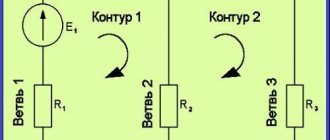
Number all nodes and set an arbitrary direction of currents in the circuit.
Pull together nodes with the same potential. The nodes will have the same potential if between them there is a pure branch with zero resistance - a short circuit (branches between nodes 2 - 4 and 3 - 5 in Fig. 1). It is not necessary to redraw the diagram with knotted nodes, but then it should be taken into account that the potentials of the nodes at the ends of the short circuit will be the same.

Rice. 1. An example of combining nodes with the same potential

Select a base node (Fig. 2) and set its potential equal to zero $ \underline_ = 0 \space \textrm $. You can choose any one as a basic node, except for the case when there are special branches. If the circuit has at least one special branch, then one of the ends of one of these branches should be taken as the basic node. In this case, the potential of the other end will be equal to the EMF $ \underline_ = \underline_ $ if the voltage source is directed to this node, and equal to minus the EMF $ \underline_ =- \underline_ $ if the source is directed to the base node.

Rice.
2. Selecting a base node Note. Often, a grounding symbol is used to designate a basic node, since it is generally accepted that “earth” has zero potential.

Compose equations for nodes without special branches, the potentials of which are unknown. The equations are written according to the following principle:

the potential of the node in question is multiplied by the sum of the conductivities of all branches adjacent to it;

the potentials of nodes located at opposite ends of adjacent branches are subtracted, each multiplied by its own conductivity of the branch connecting them;

is equated to the algebraic sum of current sources and EMF sources adjacent to a given node, the latter are multiplied by the conductivity of the branch in which they are located. The algebraic sum means the need to take into account the direction of sources; if the source is directed to the node in question, then it is written with a “+” sign, otherwise with a “-” sign.

If there is more than one special branch, and they do not have common nodes, then the equations for nodes that include a special branch that is not adjacent to the basic node are written as follows:

the potential of the node in question is multiplied by the sum of the conductivities of all branches adjacent to it and the conductivities of the branches adjacent to the node of the opposite end of the special branch;
the potentials of the nodes located at opposite ends of the adjacent branches to the nodes of a special branch are subtracted, each multiplied by its own conductivity of the adjacent branch;
is equal to the algebraic sum of current sources and EMF sources adjacent to the nodes of a special branch, the latter are multiplied by the conductivity of the branch in which they are located, with the exception of the EMF source of a special branch, which is multiplied by the sum of the conductivity of the branches adjacent to the node of the opposite end of the special branch.
When composing the equation, the conductivity of the special branch is not taken into account ( 1 /=∞). It should also be taken into account that the direction of the EMF of a special branch and, accordingly, its sign are taken into account relative to the node in question.

Calculate the currents in the branches according to Ohm's law as the algebraic sum of the potential difference and the emf in the branch with the desired current, divided by the resistance of this branch. The subtractive potential will be the one towards which the current is directed, and the sign of the EMF is selected depending on the direction: in the case of co-direction with the current, the EMF is taken with the “+” sign, otherwise with the “-” sign. The current in the short circuit should be sought according to Kirchhoff's first law, compiled for one of the nodes of the branch under consideration in the original circuit, after calculating all other currents in the circuit.
The easiest way to check the correctness of the calculation using the nodal potential method is to use Kirchhoff’s first law for unique nodes without special branches by substituting the obtained current values. By unique nodes we mean those nodes, when considering which there is at least one branch that is not adjacent to other of the considered nodes.

Example solution. As an example, consider a circuit with two special branches and a current source (Fig. 3). The number of equations compiled to find the nodal potentials is equal to

6 (total nodes) – 1 (basic node) – 2 (special branch nodes) = 3.

Let us arbitrarily designate the nodes and currents in the diagram. We take one of the nodes of one of the special branches (1-4 and 3-6) as the basic one, for example node 4, in which case $ \underline_ = 0 $, and $ \underline_ = \underline_ $.

Rice. 3. Example of electrical circuit calculation

In branch 3-6, it is necessary to find the potential of only one of the nodes (we will calculate for node 6), since the second (potential of node 3) will differ by the EMF value, i.e. $ \underline_ = \underline_— \underline_ $. Next, you need to create equations to find the remaining potentials in nodes 2, 5 and 6. It should be noted that the capacity of the branch with the current source will not affect the calculations, since the conductivity of this branch is infinitely large, and the current is set by the source itself.

$$ \begin \underline_ \cdot (\underline_ + \underline_ + \underline_)- \underline_ \cdot \underline_— \underline_ \cdot \underline_— \underline_ \cdot \underline_ = 0 \\ \underline_ \cdot (\underline_ + \underline_ + \underline_)- \underline_ \cdot \underline_— \underline_ \cdot \underline_— \underline_ \cdot \underline_ = 0 \\ \underline_ \cdot (\underline_ + \underline_ + \underline_)- \underline_ \ cdot \underline_— \underline_ \cdot \underline_— \underline_ \cdot \underline_ = \underline_ \cdot (\underline_ + \underline_) + \underline_ \end $$

Let us substitute the known potential values, reducing the number of unknowns:

$$ \begin \underline_ \cdot (\underline_ + \underline_ + \underline_)- 0 \cdot \underline_— \underline_ \cdot \underline_— \underline_ \cdot \underline_ = 0 \\ \underline_ \cdot (\underline_ + \underline_ + \underline_)- \underline_ \cdot \underline_— \underline_ \cdot \underline_— (\underline_— \underline_) \cdot \underline_ = 0 \\ \underline_ \cdot (\underline_ + \underline_ + \underline_) - \underline_ \cdot \underline_— \underline_ \cdot \underline_— \underline_ \cdot \underline_ = \underline_ \cdot (\underline_ + \underline_) + \underline_ \end $$

Let us transfer all the free components to the right side of the equalities and obtain a finite system of equations with three unknown nodal potentials:

$$ \begin \underline_ \cdot (\underline_ + \underline_ + \underline_)- \underline_ \cdot \underline_— \underline_ \cdot \underline_ = 0 \\ \underline_ \cdot (\underline_ + \underline_ + \underline_) - \underline_ \cdot \underline_— \underline_ \cdot \underline_ = \underline_ \cdot \underline_— \underline_ \cdot \underline_ \\ \underline_ \cdot (\underline_ + \underline_ + \underline_)- \underline_ \cdot \ underline_— \underline_ \cdot \underline_ = \underline_ \cdot \underline_ + \underline_ \cdot (\underline_ + \underline_) + \underline_ \end $$

To solve a system of equations with unknown nodal potentials, you can use Matlab. To do this, we present the system of equations in matrix form:

$$ \begin \underline_ + \underline_ + \underline_ & -\underline_ & -\underline_ \\ -\underline_ & \underline_ + \underline_ + \underline_ & -\underline_ \\ -\underline_ & -\underline_ & \underline_ + \underline_ + \underline_ \end \cdot \begin \underline_ \\ \underline_ \\ \underline_ \end = \\ = \begin 0 \\ \underline_ \cdot \underline_— \underline_ \cdot \underline_ \\ \underline_ \cdot \underline_ + \underline_ \cdot (\underline_ + \underline_) + \underline_ \end $$

Let's write a script in Matlab to find unknowns:

Note. To solve numerically, it is necessary to replace the symbolic assignment of variables with real values of conductivity, emf and source current.

As a result, we obtain a column vector $ \underline> $ of three elements, consisting of the desired node potentials, while the currents in the branches are through the node potentials:

To check the correctness of the calculation, you can use the equations according to Kirchhoff’s first law: if the sums of the currents in nodes 2 and 5 are equal to zero, then the calculation was performed correctly:

$$ \underline _ + \underline

_— \underline
_ = 0, $$
$$ \underline _ + \underline

_— \underline
_ = 0. $$
So, the nodal potential method allows you to calculate a smaller number of complex equations for calculating an electrical circuit in comparison with other methods with a smaller number of nodes compared to the number of circuits.

Laboratory work on electrical engineering Design protection

Laboratory work No. 1

Measuring the potentials of points in an electrical circuit

Learn to measure the potentials of points in an electrical circuit and build potential diagrams.

Experimentally verify the validity of Kirchhoff's second law.

2. Theoretical information and guidelines

The equation of Kirchhoff's second law can be represented as follows:

from which it follows that the algebraic sum of potential changes when completely circling the circuit is equal to zero.

A clear illustration of Kirchhoff's second law is a potential diagram, which makes it possible to determine the voltage drop in individual sections of an electrical circuit.

To construct a potential diagram of a closed circuit ABCDEA (Fig. 3), it is necessary to determine the potentials of individual points of the circuit.

Rice. 3. Closed loop diagram with two EMF sources

We will assume that the resistance values, magnitudes and directions of the emf E1 and E2 are known.

Point A of the circuit is connected to the ground (“grounded”) and, therefore, its potential is zero (φA = 0).

We arbitrarily select the directions of current I in the circuit and the direction of bypassing the circuit (clockwise). Let's start traversing the contour from point A in the selected direction. In this case, we pass through resistance R1 in the direction of the current. Since the current is directed from the point with the highest potential to the point with the lowest potential, the potential of point B is lower than the potential of point A by the amount of voltage drop IR1.

The potential difference φA – φB is the voltage drop between points A and B, i.e.

since φA = 0, then the potential of point B with respect to the ground

When moving from point B to point C, we pass through a source with emf E1 from the negative pole to the positive one. As a result of the action of external forces from the source, the potential of point C should increase by the amount E1. since the EMF source has an internal resistance r01, a voltage drop occurs in it I∙r01, which causes a slight decrease in the potential of point C. Therefore, the potential of point C with respect to the ground is equal to:

φC = φB + E1 – I r01 = – IR1+ E1 – I r01.

When moving from point C to point D, we pass through resistance R2 in the direction of the current, so the potential of point D is lower than the potential of point C by the amount of voltage drop IR2.

The potential of point D with respect to the ground is equal to:

φD = φC – IR2 = – IR1 + E1 – I r01 – IR2.

When moving to point E, we pass through a source with emf E2 from the positive pole to the negative. Consequently, the potential must decrease by the amount of emf E2. The presence of resistance r02 at the EMF source causes a voltage drop in it Ir02. Therefore, the potential of point E with respect to ground is equal to:

φE = φD – E2 – Ir02 = – IR1 + E1 – Ir01 – IR2 – E2 – Ir02.

From point E through resistance R3 we come to point A in the direction of the current. The potential of point A is lower than the potential of point E by the amount of voltage drop IR3, therefore:

φA = φE – IR3 = – IR1 + E1 + Ir01 – IR2 – E2 – Ir02 –IR3.

Since the potential of point A is zero (UA = 0), then

– IR1 + E1 + Ir01 – IR2 – E2 – Ir02 –IR3 = 0,

i.e., we have obtained the equation of Kirchhoff's second law for the ABCDEA contour.

This equation can be rewritten as follows:

E1 – E2 = IR1 + IR2 + IR3 + Ir01 + Ir02 =i(R1 + R2 + R3 + r01 + r02).

Where does the current in the circuit come from:

Knowing the potentials of points in the circuit and the resistance of sections, you can construct a potential diagram.

When constructing a potential diagram, the resistances between the points of the circuit are plotted along the abscissa axis, and the potentials of these points are plotted along the ordinate axis. The potential diagram for the considered electrical circuit is shown in Fig. 4.

Rice. 4. Potential diagram of the electrical circuit under consideration

A potential diagram can be constructed not only analytically, but also based on experimental data. To do this, the potentials of points in the electrical circuit are measured with a voltmeter.

Determination of electric field strength using potential