Voltage follower based op-amp

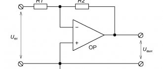
Op-amp follower circuit, powerful voltage follower on TDA2030

A voltage follower is a non-inverting amplifier with unity gain. This is realized by closing the negative feedback and supplying a useful signal to the non-inverting input.

When turned on in this way, the operational amplifier tries to provide an exact copy of the signal arriving at its input at the output. At each moment of time Uout = Uin , therefore the described circuit is called a repeater. Op-amp repeater circuit:

The meaning of using a voltage follower

Why repeat what already exists? A unity gain amplifier is also called a buffer or buffer stage. Possessing large input and low output impedances, the repeater is ideally suited for matching cascades in terms of resistance.

In this way, the main rule of circuit design is observed - the input resistance of the next stage must be at least 3, and preferably 10 times greater than the output resistance of the previous stage . In this case, the signal does not undergo distortion.

Operational Amplifier Parameters

Modern operational amplifiers have enormous input impedance. The same cheap and widespread TL062 has an input impedance of 1012 Ohms. For a dual operational amplifier (TL062, TL072, NE5532, LM833....) in a DIP-8 or SO-8 package, the repeater connection is shown below:

For operational amplifiers, as the gain increases, the frequency range narrows and the upper transmitted frequency decreases. But in repeater mode, working with unity gain, the op-amp is capable of operating up to the maximum possible frequencies for it.

One way or another, when choosing an op-amp for a repeater, it is advisable to have a frequency margin of several times, preferably 10. In this case, you can definitely not worry about any phase distortions introduced by the operational amplifier itself.

When choosing a microcircuit for a repeater, in addition to the width of the frequency range, an important characteristic is also the output current that the op-amp is capable of delivering to the load. If the operational amplifier is not able to provide the output current required by the load, then sag and distortion begin. Therefore, if we are talking about a low-impedance load that requires a current of more than 100 mA, then not every operational amplifier can handle this.

How to calculate the amount of current that the op-amp should provide?

Very simple! Let's assume that a 10 ohm resistor acts as a load. The repeater receives a voltage of 5 volts, which it must transfer to the load. In this case, applying Ohm's law (I=U/R), we find out that to maintain 5 volts across the resistor, the op-amp needs to provide a current of 0.5 amperes. (This is a rough estimate, but quite applicable in practice)

Conventional op amps will not be able to cope with this task. Of course, the output can be boosted with a transistor, but then the use of a repeater on an op-amp becomes less justified.

For such purposes, it is proposed to use TDA2030, TDA2040 or TDA2050 connected in a repeater circuit. The microcircuits are ready-made operational amplifiers equipped with transistors, which differ in maximum output power.

TDA2030 as a voltage repeater

For example, consider the TDA2030 chip, because the other two are its more powerful brothers. The microcircuit was originally developed and used in sound amplifiers. The vast majority of household amplifiers, especially 2.1 and 5.1 systems, are built on this chip. What is logical and understandable is that the chip is cheap and at the same time has good characteristics.

The microcircuit is implemented in a five-pin package and requires a minimum of parts for operation. When switched on according to a repeater circuit, only power supply capacitors are required for normal operation. It is better to also leave a resistor at the input to tie the input to ground at a constant voltage, although it is not necessary.

Standard circuit for connecting a microcircuit as an audio amplifier:

In the standard connection of the microcircuit (shown above), proposed by the data shield, the gain is set to about 20. In this case, the operating frequency band is limited by the same data shield at 140 kHz. However, when operating in a voltage follower circuit with unity gain, the microcircuit can operate up to frequencies of 0.5...1 MHz. At least the microcircuit performed well when operating at a frequency of 100 kHz, supplied from a sinusoidal signal generator on the Wien bridge, to amplify the output of which it was used.

Elegant, beautiful, and most importantly, it works. The microcircuit heats up considerably and it is advisable to use a radiator with sufficient surface area. A PC processor heatsink is perfect. However, heat dissipation depends on the operating mode and load resistance. It is not recommended to turn on the microcircuit without a heatsink.

In the original version, the microcircuit is powered by a stabilized voltage of ±9 Volts to ensure stability of the signal amplitude. The microcircuit was supposed to operate with a power of 2-3 Watts; for this reason, power stabilization was performed on banks 7809 and 7909, capable of providing current up to 1A (subject to the presence of radiators). The supply voltage range for the TDA2030 microcircuit is ±6 ... ±18 Volts .

Op amp inverting amplifier

to contents

Figure 2 shows the circuit of a simple inverting amplifier

.
The non-inverting input is grounded, i.e. is under zero voltage ( Uin2
in Figure 1 is equal to zero).
The input signal is fed through resistor R1
to the inverting input
.
The operational amplifier is covered by parallel negative voltage feedback through resistor
ROC
. Let's find an expression for the gain of the circuit.

Figure 2. Inverting amplifier

In accordance with expression (3)

UA = UB = 0 (5)

Therefore, the potential of point A

to a first approximation, it is equal to the potential of the common bus - “ground”. Therefore, this point was called “virtual land”.

Using the obtained value, we find for the currents included in (4)

; (6)

. (7)

Equating them and taking into account that K

=
Uout / Uin,
we obtain for the gain of the inverting amplifier

, (8)

where the minus sign indicates a change in the phase of the output signal compared to the phase of the input signal by 1800 (the output voltage is in antiphase, inverse, with the input voltage). In this regard, if the input signal increases, then the amplified output signal decreases, and vice versa, a decreasing input signal corresponds to an increasing output signal. We have already encountered a similar phenomenon when considering OE

,
OB
and
OI
.

From (8) it is clear that the inverting amplifier can have any gain, both greater than unity and less.

Parallel negative voltage feedback reduces the output (see (1)) and output impedance of the amplifier. The value of the latter, to a first approximation, can be determined using the concept of “virtual earth”. Since the voltage at point A

is equal to zero, then for the input signal source it “seems” that resistor
R1
, i.e.

Rin and us = R1. (9)

As shown in the previous section, the introduction of OOS

expands the range of amplified frequencies.
The figure shows the logarithmic amplitude-frequency response of an op-amp
and an inverting amplifier designed on the basis of this
op-amp
.

Figure 3. Logarithmic amplitude-frequency response of the op-amp

and inverting amplifier

Large gains of the original op-amp

correspond to a very narrow frequency range - from zero to approximately several tens/hundreds of hertz.

The flat gain of the inverting amplifier extends to the upper frequency equal to:

. (10)

to contents

Did you know,

that when some researchers trying to reconcile relativism and ethereal physics say, for example, that the cosmos consists of 70% “physical vacuum”, and 30% of matter and field, then they fall into a fundamental logical contradiction. This contradiction is as follows. Matter and field are not something separate from the ether, just as the human body is not something separate from the atoms and molecules of its components. It is these atoms and molecules assembled in a certain order. Also, matter is not something separate from elementary particles, but it consists of them as basic matter. Also, elementary particles consist of ether particles as the basic matter of the lower level. Thus, everything that exists in the universe is ether. Ether 100%. Elementary particles are made of it, and everything else is made of them. Read more in the FAQ on ethereal physics.

Operational Amplifiers: 10 Circuits for (Almost) Every Occasion

Hi all! Recently, I have mostly gone into digital and, partly, into power electronics and rarely use operational amplifier circuits. In this regard, obeying the steady law of memory half-life, my knowledge about operational amplifiers began to gradually fade, and every time I still needed to use this or that circuit with their participation, I had to Google its calculation or look for it in books. This turned out to be not very convenient, so I decided to write a kind of cheat sheet in which I reflected the most commonly used circuits on operational amplifiers, giving their calculations, as well as simulation results in LTSpice.

Introduction

This article will look at ten commonly used operational amplifier circuits. When writing this article, I assumed that the reader knows what an operational amplifier is and at least has a general understanding of how it works. It is also assumed that he knows basic electrical circuit theory, such as Ohm's law or voltage divider calculations. This article should not be taken as a complete guide to using op amps in any situation. For a large number of tasks, indeed, these schemes may be sufficient, but in complex projects something non-standard may always be required.

Non-inverting amplifier

A non-inverting amplifier is probably the most common operational amplifier circuit; it is shown in the figure below.

In this circuit, the amplified signal is fed to the non-inverting input of the operational amplifier, and the output signal is fed through a voltage divider to the inverting input. The calculation of this circuit is simple, it is based on the fact that the operational amplifier, covered by a feedback loop, processes the input effect in such a way that the voltage at the inverting input is equal to the voltage at the non-inverting input: From this formula, the gain of the non-inverting amplifier is easily obtained: Let's calculate and simulate non-inverting amplifier with the following parameters:

• Operational amplifier LT1803
• Gain
• Input frequency
• Input amplitude
• DC component of the input signal

Let's choose from the range E96 and. Then the gain will be equal to The result of modeling this circuit is shown in the figure (picture clickable):

Let's now look at the edge cases of this amplifier. Let's say the value of the resistor is . In this case, we find that the gain will tend to infinity. In fact, of course, although this is a very large, it is still a finite value; it is usually given in the documentation for the chip of a specific operational amplifier. On the other hand, the output voltage of a real operational amplifier, even with an infinitely large gain, cannot be infinitely large: it is limited by the supply voltage of the microcircuit. In practice, it is often even somewhat less, with the exception of some types of amplifiers that are marked as rail-to-rail. But in any case, it is not recommended to drive operational amplifiers to their limiting states: this leads to saturation of their internal output stages, nonlinear distortions and overloads of the microcircuit. Therefore, this limiting case does not have any practical benefit. Of much greater interest is another limiting case, when the resistance value is . We will look at it in the next section.

Repeater

As mentioned earlier, turning on an operational amplifier in a repeater circuit is the limiting case of a non-inverting amplifier, when one of the resistors has zero resistance. The repeater circuit is shown in the figure below.

As can be seen from the formula given in the last section, the transmission coefficient for a repeater is equal to one, that is, the output signal exactly repeats the input signal. Why do you need an operational amplifier in this case? It acts as a buffer, having a high input impedance and a low output impedance. When is this necessary? Let's say we have some kind of signal source with a high output impedance and want to transmit this signal without distortion to a relatively low-impedance discharge. If we do this directly, without any buffers, we will inevitably lose some part of the signal. Let's verify this by simulating a circuit with the following main parameters:

• Signal source output impedance 10 kOhm
• Load resistance 1 kOhm
• Input frequency
• Input amplitude
• DC component of the input signal

We will carry out simulations for two cases: in the first case, let the signal source operate to the load through a repeater, and in the second case, directly. The simulation results are shown in the figure below (the picture is clickable): on the top oscillogram, the output and input signals exactly coincide with each other, while on the bottom, the output signal is several times smaller in amplitude relative to the input signal.

Instead of a follower on an operational amplifier, you can also use an emitter follower on a transistor, without forgetting, however, about its inherent limitations.

Inverting amplifier (classical circuit)

In the inverting amplifier circuit, the input signal is supplied to the inverting pin of the microcircuit, and feedback is also connected to it. The non-inverting input is connected to ground (sometimes to a bias source). A typical inverting amplifier circuit is shown in the figure below.

For the input circuit of the inverting amplifier, you can write the following expression: Where is the voltage at the inverting input of the operational amplifier. Since the operational amplifier, covered by a feedback loop, strives to equalize the voltages at its inputs, then, and with a grounded non-inverting input, we obtain. Hence, the gain of the inverting amplifier is equal. For the inverting amplifier, the following conclusions can be drawn:

1. An inverting amplifier inverts the signal. This means that it is necessary to use bipolar power.
2. The magnitude of the gain of the inverting amplifier is equal to the ratio of the feedback circuit resistors. If the values ​​of two resistors are equal, the gain is -1, i.e. An inverting amplifier simply works as a signal inverter.
3. The value of the input resistance of the inverting amplifier is equal to the value of resistor R1. This is important because with small values ​​of R1 the previous stage can be heavily loaded.

For example, let's calculate an inverting amplifier with the following parameters:

• Operational amplifier LT1803
• Gain
• Input frequency
• Input amplitude
• DC component of the input signal

As resistors in the feedback circuit, we will choose resistors with nominal values ​​and: their ratio is exactly equal to ten. The results of amplifier modeling are shown in the figure (picture clickable).

As you can see, the output signal is 10 times larger in amplitude than the input signal, and at the same time it is inverted. The input impedance of this circuit is . What will happen if the signal source has a significant output impedance, say the same 10 kOhm? The result of modeling this case is presented in the figure below (the picture is clickable).

The amplitude of the output signal dropped by half compared to the previous case! Obviously, this is all due to the fact that the output impedance of the generator in this case is equal to the input impedance of the inverting amplifier. Thus, it is worth always remembering this feature of the inverting amplifier. What to do if you still need to ensure the operation of a signal source with a high output impedance to an inverting amplifier? In theory, you need to increase the resistance R1. However, at the same time, resistance R2 will also increase. If we want to provide a circuit input impedance of 500 kΩ at a gain of 10, resistor R2 must have a resistance of 5 MΩ! It is not recommended to use such large resistance values: the circuit will be very sensitive to interference, dust and flux on the printed circuit board. Are there any ways out of this situation? Actually yes. You can, for example, use a repeater buffer, which we discussed in the last section. You can also use a circuit with a T-shaped bridge in feedback, we’ll talk about it in the next section.

Inverting amplifier with T-bridge in the OS circuit

The circuit of an inverting amplifier with a T-shaped bridge in the feedback circuit is shown in the figure below.

The gain of this circuit is Calculate an amplifier with the following parameters:

• Operational amplifier LT1803
• Gain
• Input frequency
• Input amplitude
• DC component of the input signal
• Input impedance

The calculation shows that the tracking resistor values ​​should form an amplifier with a T-bridge that meets the stated requirements: The results of modeling the amplifier circuit are shown in the figure below (picture clickable).

Let's now try to connect a source with an output impedance of 10 kOhm, as we did in the previous section. We get this picture (clickable):

The output signal remained virtually unchanged in amplitude compared to the previous simulation, and this cannot be compared to how much it sagged in the circuit of a simple inverting amplifier without a T-bridge. In addition, as we see, this circuit allows you to do without megaohm resistors even with high gains and significant input resistance.

Inverting amplifier in single-supply circuits

Single-supply circuits are much more common than dual-supply circuits. At the same time, as we found out in the previous two sections, when using an inverting amplifier circuit, the sign of the output voltage changes, which entails the mandatory use of a bipolar power supply. Is it possible to somehow get around this limitation and use an inverting amplifier in single-supply circuits? In fact, it is possible, to do this you need to apply a bias voltage to the non-inverting input of the amplifier as shown in the figure below

Note

Positional designations R1 and R2 are shown conventionally.
They are the same for different resistors in the circuit, which, of course, is impossible for a real circuit, but is allowed in the figure to emphasize that these resistors have the same values. The calculation of this circuit is based on the same principle of equality of voltages at the inverting and non-inverting inputs of the amplifier. The current through the chain of resistors R1-R2 of the inverting arm is equal. Hence, the voltage at the inverting input is equal. The voltage at the non-inverting input is equal. Based on the principle of equality of the voltage at the inverting and non-inverting inputs, we obtain Thus, the voltage at the output of the operational amplifier is equal. Hence we conclude that for correct operation of the voltage The offset must be greater than the maximum input voltage, taking into account the offset voltage applied to the input. Let's simulate an inverting amplifier circuit with the following parameters:

• Operational amplifier LT1803
• Gain
• Input frequency
• Input amplitude
• DC component of the input signal
• Bias voltage

The simulation results are shown in the figure below (picture clickable)

As you can see, we received an inverted signal amplified by 10 times, while the signal was inverted, however, it did not go into the negative region.

Inverting adder

An operational amplifier can be used to sum various signals. Using resistors, you can set the “weight” of each signal in the total. The inverting adder circuit is shown in the figure below.

The calculation of the inverting adder is very simple and is based on the principle of superposition: the total output signal is equal to the sum of the individual components: Let's calculate and simulate the inverting adder with the following parameters:

• Operational amplifier LT1803
• Input frequency
• Input signal amplitude #1
• Input signal amplitude #2
• Input signal amplitude #3
• "Weight" of signal No. 1
• “Weight” of signal No. 2
• “Weight” of signal No. 3

To provide the required “weights”, we will select the appropriate resistor values ​​from the E96 series: The simulation result is shown in the figure below (the picture is clickable).

We see that the output signal is inverted and amplified in accordance with the expression given above. However, it is always worth remembering that the above expression is true for constant voltages (or instantaneous values ​​of an alternating signal). If the signals are shifted in phase or if they have different frequencies, the result will be completely different. It can be calculated analytically using formulas for converting trigonometric expressions (if we are dealing with sinusoidal signals). As an example, the figure below shows the result of modeling an inverting adder for the case of phase-shifted input signals (clickable image).

As we can see, the final signal does not exceed the signal in amplitude, and also has artifacts in the initial part caused by the gradual appearance of signals at the inputs. It is also necessary to remember that the inverting adder is essentially the same inverting amplifier, and its input resistance is determined by the value of the resistor in the feedback circuit, so it must be used carefully in cases where the signal source has a high output impedance.

Differential amplifier

A differential amplifier is designed to amplify the difference in signals arriving at its inputs. This connection of amplifiers is widely used, for example, to amplify the signal from a resistor-shunt-current sensor. What is important is that the operational amplifier in such a connection, in addition to actually amplifying the signal, suppresses common-mode interference. The differential amplifier circuit is shown in the figure.

For a differential amplifier, the following expressions can be written:

Solving this system of equations, we get If we accept that then this expression is simplified and transformed into Thus, the gain of the differential signal is determined by the ratio of R2 to R1. This formula (and the differential amplifier circuit itself) is very similar to the previously discussed case of an inverting amplifier in a single-supply circuit. Indeed, everything is so: the circuit of an inverting amplifier with a unipolar supply and a bias voltage is a special case of a differential amplifier, it’s just that in it, not some kind of alternating signal, but a constant voltage is supplied to one of the inputs. Let's simulate the circuit with the following parameters:

• Operational amplifier LT1803
• Gain
• Input frequency
• Input signal amplitude #1
• Input signal amplitude #2
• Magnitude of amplified signal

The simulation results are shown in the figure below (clickable image).

As you can see, the difference between the signals and 5 mV turned out to be amplified 50 times and became 250 mV. Let's now see how a differential amplifier suppresses common-mode interference. To do this, we will connect a general white noise generator to the signals and perform a simulation; its results are presented in the figure (the picture is clickable).

The upper oscillogram shows signals with added noise: the signal itself is no longer even visible behind the noise. The lower oscillogram shows the result of the differential amplifier. Since the noise is the same for the inverting and non-inverting inputs, the differential amplifier removes it, and as a result we have a clean signal, no different from the case without noise. However, it is still worth remembering that the ability of an operational amplifier to suppress common-mode noise is not infinite; this parameter is usually given in the documentation for the operational amplifier. In addition, we must not forget about the value of the input resistance of the differential amplifier on the side of the inverting input: it can still be small.

Current source

An operational amplifier, when turned on in a certain way, can act as a current source. The current source maintains a constant current regardless of the value of the load resistance (in an ideal source, the load can be any at all, in a real one - no more than any value proportional to the maximum possible voltage that the current source can generate on it). There are at least two op-amp current source circuits possible: floating load and grounded load. The circuit of a current source with a floating load is extremely simple and is shown in the figure below. As you can see, a reference voltage is supplied to the non-inverting input, and one of the feedback elements acts as a load. The magnitude of the current is determined by the following expression. However, it is still more often required that the load be grounded. In this case, the circuit becomes a little more complicated: an additional transistor is required. For these purposes, it is better to take a field-effect transistor: for a bipolar transistor, the collector and emitter currents are slightly different due to the base current, which will lead to less stable operation of the current source. The operational amplifier current source circuit with a grounded load is shown in the figure below.

The current value is calculated as follows: Let us calculate and simulate a current source with the following parameters:

• Operational amplifier LT1803
• Current value
• Load resistance value

To ensure the specified characteristics, the following resistor resistance values ​​are suitable: The result of modeling a current source with the specified parameters is presented in the figure below (clickable image).

The figure shows two graphs. The top graph shows the amount of current through the load resistance, and it is equal to 10 mA. The bottom graph shows the voltage across the load, it is equal to 100 mV. Let's now try to change the load resistance: instead of 10 Ohms, let's take 100 Ohms and simulate (clickable image):

As we can see, the same current of 10 mA flows through the load: the operational amplifier has processed the change in the load, increasing the voltage on it, it has now become equal to 1 V. But in reality, the operational amplifier will not be able to raise the voltage indefinitely: it is limited by the voltage of the power source (and often even slightly less than that). What happens if you set the load resistance too high? Essentially, the current source stops working. The figure below shows an example of modeling a source with a load resistance of 1 kOhm (clickable image).

According to the graph, the current through the load is no longer 10 mA, but only 4 mA. As the load resistance further increases, the current will become less and less. Additionally, according to the above circuits of current sources on operational amplifiers, it should be noted that the stability of the output current in them depends on the stability of the voltage, and therefore it must be well stabilized. There are more complex schemes that allow you to get away from this dependence, but we will not consider them within the scope of this article.

Operational amplifier integrator

I think that all readers are familiar with the classic integrator circuit on an RC circuit: This circuit is extremely widely used in practice, but it has one serious drawback: the output resistance of this circuit is high and, as a result, the input signal can be significantly attenuated. To eliminate this drawback, it is possible to use an operational amplifier. The simplest operational amplifier integrator circuit, found in all textbooks, is shown in the figure below.

As can be seen from the figure, this is an inverting integrator, i.e. In addition to integrating the signal, it also changes its polarity. It should be noted that this is not always required. Another serious drawback of this circuit is that the integrator capacitor accumulates a charge that must be discharged somehow. To do this, you can either use a resistor connected in parallel with the capacitor (however, its effect on the final signal must also be taken into account), or you can reset the charge using a field-effect transistor, opening it at the right times. For this reason, I decided to look in more detail at another integrator circuit using an operational amplifier, which, in my opinion, deserves more practical interest: As can be seen from the figure, this circuit is a classic RC integrator, to which an operational amplifier follower is added : It solves the problem of output impedance. An integrator can also be thought of as a low-pass filter. The cutoff frequency of the filter's frequency response is calculated using the formula. Here it is worth paying attention to one very important point. We must always remember that the cutoff frequency calculated above is only valid for the RC circuit and does not take into account the frequency properties of the operational amplifier itself. The frequency properties of an operational amplifier can be neglected if we fall within its operating frequency range, but if we suddenly go beyond it, the final frequency response of the circuit will not be at all what we expected. Roughly speaking, if our RC chain is set to 1 MHz, and the operational amplifier allows operation up to 100 MHz, everything is fine. But if we have a 10 MHz chain, and the operational amplifier operates up to 1 MHz, everything is bad. As an example, let’s calculate a low-pass filter with the following parameters: the frequency response cutoff frequency is 1 MHz. For this frequency you can choose

• Frequency response cutoff frequency
• Operational amplifier LT1803 (Maximum frequency 85 MHz)

For a given frequency response cutoff frequency, the following resistance and capacitance values ​​of the RC circuit are suitable: The simulation result is shown in the figure below (clickable image). This figure shows two frequency characteristics: separately for the RC chain (red line) and for the entire circuit (RC chain + op-amp, green line).

As can be seen from the figure, the red and green lines initially coincide, and starting from a certain frequency the green line goes down much steeper. This is precisely explained by the fact that the operational amplifier itself begins to influence the frequency properties of the circuit. Well, since we are still considering an integrator, the following figure (clickable) shows a classic picture from textbooks: integration of rectangular pulses. The integrator parameters are the same as in the previous frequency response simulation.

Operational amplifier differentiator

The circuit of the simplest differentiator on an RC circuit is no less known than the integrator circuit: This circuit has the same disadvantage associated with high output resistance, and to eliminate it, an operational amplifier can be used in a similar way. The inverting differentiator circuit is obtained from the inverting integrator circuit by replacing capacitors with resistors and resistors with capacitors, it is shown in the figure below.

However, even in this case, let us consider in more detail another circuit consisting of a classic differentiator on an RC chain and a repeater on an operational amplifier:

If we considered the integrator as a simple low-pass filter, then the differentiator, on the contrary, is a high-pass filter. The cutoff frequency of the frequency response is calculated using the same formula. In the case of a differentiator, we also must not forget about the frequency properties of the operational amplifier itself: here they are expressed even more clearly than in the case of an integrator. As we saw in the last section, from a certain frequency, the op-amp acts as a low-pass filter, while the differentiator acts as a high-pass filter. Together they will work as a bandpass filter. As an example, let’s calculate a high-pass filter with a frequency response cutoff frequency equal to the same 1 MHz. For such a frequency, you can choose all the same component values ​​that were in the case of the low-pass filter: The simulation result is shown in the figure below (the picture is clickable). This figure shows two frequency characteristics: separately for the RC chain (red line) and for the entire circuit (RC chain + op-amp, green line).

As can be seen from the figure, the red and green lines initially coincide, and starting from a certain frequency, the green line goes sharply downward, while the red line, reflecting the operation of the RC circuit itself, is horizontal. The operation of a differentiator when rectangular pulses are applied to its input is shown in the figure below (clickable image).

Conclusion

In this article, we looked at ten of the most common operational amplifier circuits.
An operational amplifier is a powerful tool in the right hands, and the number of circuits that can be created with its help, of course, is many times greater than what was discussed, however, I hope this material will be useful to someone and will help to use this component more confidently in their developments. useful links

1. Horowitz P., Hill W. The Art of Circuit Design: - Ed. 2nd. - M.: BINOM Publishing House - 2014. - 704 p.
2. Carter B., Mancini R. Operational amplifiers for everyone - M.: Publishing house "Dodeka - XXI" - 2011. - 509 p.
3. LT1803