Self-excitation of a parallel excitation generator
Self-excitation of the parallel excitation generator occurs when the following conditions are met: 1) the presence of residual magnetic flux of the poles; 2) correct connection of the ends of the field winding or the correct direction of rotation. In addition, the resistance of the excitation circuit Rв at a given rotation speed n must be below a certain critical value, or the rotation speed at a given Rв must be higher than a certain critical value.
For self-excitation, it is enough that the residual flow is 2 - 3% of the nominal one. A residual flow of this value is almost always present in a machine that has already been running. A newly manufactured machine or a machine that has become demagnetized for some reason must be magnetized by passing current from an external source through the field winding.
If the necessary conditions are met, the self-excitation process proceeds as follows. A small electromotive force (emf), induced in the armature by the residual magnetic flux, causes a small current iв in the field winding. This current causes an increase in the flux of poles, and therefore an increase in e. d.s., which causes a further increase in iв, and so on. This avalanche-like self-excitation process continues until the generator voltage reaches a steady value.
If the connection of the ends of the field winding or the direction of rotation is incorrect, then a current i in the opposite direction occurs, causing a weakening of the residual flux and a decrease in e. d.s., as a result of which self-excitation is impossible. Then it is necessary to switch the ends of the field winding or change the direction of rotation. You can verify that these conditions are met by monitoring the armature voltage with a voltmeter with a small measurement limit when closing and opening the excitation circuit.
The polarity of the generator terminals during self-excitation is determined by the polarity of the residual flow. If, for a given direction of rotation, the polarity of the generator needs to be changed, then the machine should be remagnetized by supplying current to the field winding from an external source.
Figure 1. Self-excitation of a parallel excitation generator at different excitation circuit resistances (a) and at different rotation speeds (b)
Let's take a closer look at the process of self-excitation at idle. In Figure 1, a, curve 1 represents the idle speed characteristic (x. x. x.), and straight line 2 is the so-called excitation circuit characteristic or the dependence Uв = Rв × iв, where Rв = const is the resistance of the excitation circuit, including the resistance of the adjusting rheostat.
During the process of self-excitation iв ≠ const and the voltage at the ends of the excitation circuit
where Lв is the inductance of the excitation circuit.
Armature voltage at no-load (I = 0)
Uа = Eа – iв × Rа
is depicted in Figure 1, and curve 1. Since the current iв is small, then practically Ua = Ea.
But in a parallel excitation generator (see Figure 1, b, in the article “General information about direct current generators”) Uа = Uв. Therefore, the difference between the ordinates of curve 1 and straight line 2 in Figure 1, a is d(Lвiв)/dt and characterizes the speed and direction of change of iв. If line 2 passes below curve 1, then
iв grows and the machine self-excites to the voltage corresponding in Figure 1, and the point of intersection of curve 1 and straight line 2, at which
and the growth of iв therefore stops.
From an examination of Figure 1, a, it follows that the increase in iв and, therefore, Ua occurs slowly at first, then accelerates and slows down again towards the end of the process. The self-excitation process that has begun stops or is limited at point a' due to the curvilinearity of x. X. X. In the absence of saturation, Ua would theoretically increase to Ua = ∞.
In general, any self-excitation processes - electrical, and others, observed in various devices - are limited only by the nonlinearity of the system characteristics.
| Figure 2. Magnetic saturation bridges in a magnetic circuit |
If Rв is increased, then instead of straight line 2 we get straight line 3 (Figure 1, a). In this case, the self-excitation process slows down and the machine voltage, determined by point a'', will be less. With a further increase in Rv, we obtain straight line 4, tangent to curve 1. In this case, the machine will be on the verge of self-excitation: with small changes in n or Rv (for example, due to heating), the machine can develop a small voltage or lose it. The value of Rв, corresponding to line 4, is called the critical resistance of the excitation circuit (Rв.кр). When Rв > Rв.кр (straight line 5), self-excitation is impossible and the machine voltage is determined by the residual flux.
From the above it follows that the parallel excitation generator can only operate if there is a certain saturation of the magnetic circuit. By changing Rв you can adjust U to the value U = Umin, corresponding to the beginning of the knee of the x curve. X. X. In conventional machines Umin. = (0.65 – 0.75)Un.
E.m.f. Ea ∼ n, and for different values n1 > n2 > n3 we obtain x. X. x., shown in Figure 1, b by curves 1, 2, 3. From this figure it is clear that with a small value of Rв in the case of curve 1 there is stable self-excitation, with curve 2 the machine is on the verge of self-excitation and with curve 3 self-excitation is impossible. Therefore, for each given value of Rв there is such a value of rotation speed n = ncr. (curve 2 in Figure 1, b), below which self-excitation is impossible. This value is n = ncr. called the critical rotation speed .
| Figure 3. Parallel excitation generator no-load characteristics |
In some cases, it is required that U of the parallel excitation generator can be adjusted within wide limits, for example Un: Umin. = 5 : 1 or even U : Umin. = 10:1 (synchronous machine exciters). Then the curve x. X. X. should be bent already in its initial part. For this purpose, if necessary, sections with a weakened cross-section (magnetic saturation bridges) are made in the magnetic circuit in the form of slots in the sheets of the pole cores (Figure 2, a), protrusions in the upper part of these sheets (Figure 2, b) and the like. In such bridges, the magnetic flux is concentrated, and their saturation occurs even at low fluxes.
Operating characteristics of the independent excitation generator.
External characteristics
—
U=f(I)
with
I
in = const and
n
= const.
To remove the external characteristic, it is necessary to rotate the generator at the rated speed and set the excitation current I
in such that at
I= IH= Os
(Fig. 4.13) there is a rated voltage at the generator terminals
UH= Ca = OB.
Then the generator is gradually unloaded to idle speed.
Voltage; at the generator terminals it increases and at I
= 0 reaches the value
Uo = OA.
Hence,
(4.11)
An external characteristic can be constructed using the idle characteristic and the short circuit triangle.
Rice. 4.12. External characteristics of the independent excitation generator
Rice. 4.13. Construction of an external characteristic of an independent excitation generator
Rice. 4.14. Regulating characteristics of the independent excitation generator
Let the generator excitation current I
c, which remains a constant value, is given by the segment
Oa
(Fig. 4.11).
From point a
we draw a straight line parallel to the ordinate until it intersects with the idle speed characteristic at point
b.
Then
ab
=
Eа0 = Uo,
where
Ea0 is
the EMF, and
Uo is
the voltage at the generator terminals at idle.
Let us construct from point a a
short-circuit triangle
aA'B',
corresponding to some current
I
, for example
I
=
I
nom.
direct leg aB' = IHRa
along line
ab
and force triangle A'B'a
to slide along it, parallel to itself, until point A
falls
A'B'a
takes the position of triangle ABC
,
The segment
Oa'
represents the resulting MMF of the machine, i.e.
MMF of the main poles Oa,
reduced by the value of the demagnetizing MMF of the armature
aa'.
The segment
a'A
=
AB
determines the emf of the generator at a given load, and the segment
aC = aB - BC
determines the voltage at the generator terminals
U
at
I
=
I
n.
To get the voltage U
for other currents, for example
I
= 0.5
I
nom, you need to do the same construction, reducing all sides of the short circuit triangle by 2 times.
For simplicity, you can divide the segment aa'
in half, move point
a" to
point
A
on the idle characteristic and then draw straight line
A1C1
parallel to the hypotenuse
AC.
The segment
Ac1
will give the desired voltage
U
at
I
= 0.5
I
nom.
I on a given scale
= 0, 0.5
Inom
,
Inom
, etc. to the left of the ordinate axis and move the corresponding points b1,
C1,
C to points
d0, d1, d.
Then the
dod1d
will represent the external characteristic of the generator.
Rice. 4.15. Construction of the regulating characteristic of an independent excitation generator
Regulating characteristic - I
в =
f
(
I
) with
U =
const and
n
= const.
Since the voltage at the generator terminals increases as the load decreases, in order to maintain it constant, it is necessary to reduce the excitation current Iv
.
An approximate adjustment characteristic is shown in Fig. 4.14. It can be constructed in the same way as the external characteristic, based on the idle characteristic and the short circuit triangle. To do this, draw the DC
parallel to the abscissa axis at a distance of 0
D
=
Unom
from the latter (Fig. 4.16).
Having constructed a short circuit triangle ABC
for some, for example rated, current, we position this triangle so that vertex
A
lies on the no-load characteristic, and vertex C lies on the straight line
DC;
the excitation current
I
required to create voltage
Un .
Moving point a
down from the x-axis according to the current
I
nom, we obtain point
N
of the control characteristic corresponding to the rated load.
Other points of the control characteristic are also constructed, for example, point
M
for
I
=
0.5
I
nom, while all sides of the short circuit triangle change in proportion to the current
I. For idle speed Iв0
=0a0. The adjustment characteristic is determined by the
NMa0 curve.
Rice. 4.16. Load characteristics of the independent excitation generator
1 - idle speed characteristics; 2-load characteristic
Load characteristics - U
=
f
(
I
in) with
I
= const and
n
= const.
The voltage at the generator terminals is always less than the EMF due to the voltage drop in the armature and the reaction of the armature. When I
= const, the action of these two factors is almost constant, therefore the load characteristic (curve
2
in Fig. 4.16) is located almost parallel to the idle characteristic.
Just like other stroke characteristics, load characteristics can be constructed based on the idle characteristic and the short circuit triangle. Since I =
const, when constructing it is necessary to move the short circuit triangle ABC
parallel to itself, sliding the vertex A
along
Characteristics of the parallel excitation generator. The parallel excitation generator (see Fig. 4.2) operates with self-excitation. To do this, it is necessary that the generator has a small (2...5% of the nominal) residual magnetization flux Fost. If, by closing the excitation circuit, the generator is rotated at a certain, for example, rated speed, then a small voltage will appear at its terminals and a current will flow through the excitation circuit, which will create an additional magnetization flux Fdob. Depending on the direction of the current in the excitation winding, the flow Fdob can be directed either counter to the flow Fost, or in accordance with it. The generator can self-excite only if the direction of both flows is consistent. In other words, the process of self-excitation of the generator can go in one direction, determined by the direction of the flow Fost.
When the direction of both flows is consistent, the resulting excitation flow increases; this leads to an increase in the EMF induced in the armature and, in turn, causes a further increase in the current and excitation flux.
Let us find out the limit to which the process of self-excitation goes. In this case, we will assume that the generator is running idle, i.e. I
= 0. During self-excitation, the EMF equation of the excitation circuit can be written in the following form:
, (4.11)
or
(4.12)
where u
0 - alternating voltage at the generator terminals and, consequently, at the excitation circuit terminals;
RB
—excitation circuit resistance;
LB
is the inductance of the excitation circuit.
If RB =
const, then the voltage drop
IBRB
changes in direct proportion to the current
Iv
.
Graphically it is depicted by straight line 1 in Fig.
4.17, going at an angle α to the abscissa axis, and tan α = IBRB/IB
=
R.B.
(4.14)
Therefore, for each value of RB
corresponds to a straight line emerging from the origin at an angle determined by formula (4.14).
In Fig. 4.17 the idle speed characteristic is reflected by curve 2.
The ordinate segments between curves
2
and
1
give the difference
u
0 -
IBRB
=
d(LBIB)/dt;
and serve as a measure of the intensity of the ongoing process of self-excitation.
Obviously, this process will end when the difference u
0 –
I
B
R
B becomes equal to zero, in other words, when characteristics 1 and 2 intersect.
Thus, the steady-state value of the current I
in is determined by the intersection point
A
of characteristics
1 and 2 .
Rice. 4.17. Graphic justification for self-excitation of a parallel excitation generator:
1,3,5 - dependences of U0 on Iв at different Rв; 2.4 - characteristics of idle speed at different n
Rice. 4.18 Parallel excitation generator no-load characteristics
1- with increasing current Iv; 2 – with a decrease in current Iv; 3 – average.
If you increase the resistance RB,
those.
angle α (curves 3
and
4)
, then point
A
will slide along the idle characteristic in the direction to point
O.
With a certain resistance
R
v.kr, which is called critical resistance, straight line
1
will be tangent to the initial part of the idle characteristic (Fig. 4.17 , straight
3).
Under these conditions, the generator is practically not excited.
Since at given voltage scales u0
and current
I
V, the slope of the no-load characteristic depends on the armature rotation frequency, it is obvious that each of them has its own critical resistance
Rv.cr.
So, for example, for idle speed characteristic
4,
corresponding to a higher rotation speed, the critical resistance is determined by straight line 5.
Idle characteristic - U0 = f(IB)
for
I
a = 0 and
n =
const. This characteristic is removed in the same way as with independent excitation. However, self-excitation of the parallel excitation generator is possible only in one direction. Therefore, the idle characteristics of this generator can also be taken only with one direction of the excitation current (Fig. 4.18).
Since when the parallel excitation generator is idling, current Ia
=
I
V, then an armature reaction appears in the generator and a voltage drop occurs.
But the current Iv
usually does not exceed 2... 3%
Inom
.
Therefore, the idle characteristic taken with self-excitation practically
coincides with the corresponding characteristic with independent excitation.
External characteristic - U=f(I)
with
RB =
const and
n =
const.
In Fig. 6.61, curve 1
represents the external characteristic of the parallel excitation generator, and curve
2
is the external characteristic of this generator when operating with independent excitation.
When operating with self-excitation, the voltage drop occurs faster with increasing load. This is explained by the fact that with an increase in the load of the parallel excitation generator, in addition to the armature reaction and the voltage drop in the armature, there is also a decrease in the excitation current I
V =
U/RB = U,
which entails a decrease in the flux and a corresponding decrease in the EMF and voltage at generator terminals.
Rice. 4.19 External characteristics of the generator:
1- parallel excitation; 2- independent excitation
In Fig. 4.19 it can be seen that if you increase the load above the rated load in the independent excitation generator, then the voltage change will go along line 2; short circuit ( UK
= 0) the current in the armature
Ik
will be unacceptably large and can damage the armature winding.
When working with self-excitation (see Fig. 4.19, curve 1)
load will increase only to a critical value
I
cr, usually not exceeding the rated current by more than 2-2.5 times, and then the current
I
begins to decrease.
During a short circuit, U =
0 and
Iv
= 0, and a current
I
cost flows through the armature, determined only by the flow Fost.
Usually Ik.ost
<
Inom.
Consequently, for a parallel excitation generator, a short circuit is dangerous mainly from the point of view of switching conditions when passing through the critical current, but it is still less dangerous than for an independent excitation generator.
Increasing voltage value ΔU
The nominal to open circuit voltage at the terminals of the parallel excitation generator is much greater than in the independent excitation generator and, depending on the degree of saturation of the machine, reaches 30...35% or more.
The construction of the external characteristic of the parallel excitation generator is carried out in the same way as for the independent excitation generator, with the only difference that in the independent excitation generator the excitation current is i
in does not depend on the voltage at the terminals of the generator
U,
and in the self-excitation generator the current
I
in changes proportionally to the voltage
U.
Accordingly, the dependence
I
in
= f (U)
is depicted in Fig.
4.13 straight line ab
parallel to the ordinate axis, and in Fig.
6.62 - straight line Ob
taken from the origin at angle α, and tan α =
RB.
Therefore, the short circuit triangle
ABC
in the first case is placed between the idle characteristic and the straight line
ab,
and in the second - between the same characteristic and the straight
Ob.
Rice. 4.20. Construction of an external characteristic of a parallel excitation generator
To the left of the y-axis in Fig. 4.20 the external characteristic is plotted point by point for I
= 0,
I
= 0.5
I
nom and
I
=
I
nom.
To obtain the critical current I
MN
parallel to the straight line
Ob
to the no-load characteristic and, at the point of tangency
Ap
, draw a straight
line ApSp
parallel to the hypotenuse
AC
of triangle ABC
Then
I
cr =
IH0M((ApSp)/AC).
The control characteristics for generators with independent and parallel excitation are the same. The same applies to load characteristics.
Sequential excitation generator. Since in a series excitation generator the excitation winding is connected in series with the armature (see Fig. 4.3), the excitation current of this generator is equal to the load current I
. Consequently, the idle characteristics of the generator and its load characteristics can only be measured using a circuit with independent excitation. To do this, you need to disconnect the field winding from the armature and power it from an external source of direct current. The characteristics are as shown in Fig. 4.9.
With independent excitation, the short circuit characteristic is also removed. Using it you can construct a short circuit triangle (see Fig. 6.53). Having the idle characteristic and the short circuit triangle, it is possible to construct an external characteristic, i.e., the dependence U
=
f
(
I
) for
n
= const.
Indeed, let curve 1
in Fig.
4.21 represents the idle speed characteristic.
a short circuit triangle
A'B'C'
from point C' for some load current, for example
I
=
I
nom, and move it parallel to the ordinate axis until it takes the position of triangle
ABC
with the vertex
And
on the idle speed characteristic.
Then point C will be the point of external characteristic.
will
assume that the sides of the triangle A'B'C'
change in proportion to the current
I. Then the geometric location of points A'
is determined by straight line
2.
We make a similar construction for other currents, for example
I
= 0.5
I
nom and 0.25
I
nom.
Connecting points C, C1
and
C2,
we obtain curve
3,
which represents the external characteristic of the series excitation generator.
Mixed excitation generator. Since the mixed excitation generator has parallel and series field windings, it combines the properties of generators of both types. Typically, both windings are switched on in accordance, with the parallel winding creating the rated voltage at the terminals of the mixed excitation generator when it is idling, and the series winding compensating for the MMF of the armature reaction and the voltage drop in the armature at a certain load. This achieves automatic regulation of the generator voltage within certain load limits.
Knowing the characteristics of parallel and series excitation generators, it is easy to explain the characteristics of a mixed excitation generator. So, for example, at idle, the load current, and therefore the current of the series winding, is zero. Therefore, the no-load characteristic of a mixed excitation generator is no different from the corresponding characteristic of a parallel excitation generator.
The load characteristics of a mixed excitation generator have the same form as the corresponding characteristics of a parallel excitation generator or an independent excitation generator, but they can be located above the idle characteristics, since the voltage in the mixed excitation generator is U
under load it may be greater (with overcompensation) than at idle.
Of greatest interest is the external characteristic of the mixed excitation generator, i.e. dependence U
=
f
(
I
) for
n =
const and
Rв =
const.
Let us calculate the series winding of the generator so that it can compensate for the reaction of the armature and the voltage drop in the armature at I
=
I
nom.
In this case, the generator is called normally compensated; its external characteristic has the form of curve 2, shown in Fig. 6.64. However, more often it is necessary to maintain a constant voltage not at the terminals of the generator, but at the power receivers, for which it is necessary to additionally compensate for the voltage drop in the line. In this case, the generator is called overcompensated and its external characteristic takes the form of curve 2
shown in Fig.
4.22. For comparison, in Fig. Figure 4.22 also shows the external characteristic of the parallel excitation generator (curve 3)
and the external characteristic of the mixed excitation generator with counter-connection, i.e.
counter-connection of both excitation windings (curve 4).
Rice. 4.22 External characteristics of the mixed excitation generator:
1-normally compensated; 2-overcompensated; 3- external characteristic of the parallel excitation generator; 4 – external characteristic of a mixed excitation generator with back-switching
Rice. 4.23 Regulating characteristics of the mixed excitation generator:
1-normally compensated; 2-overcompensated.
According to external characteristics 1 and 2 shown in Fig. 4.22, the adjustment characteristics of the mixed excitation generator have the form of curves 7 and 2,
presented in Fig. 4.22.
Mixed excitation generators are used in cases where it is necessary to maintain a constant voltage U
under sharply variable load.
Short circuit characteristic
The short circuit characteristic I = f(iв) at U = 0 and n = const for a parallel excitation generator can only be removed when the excitation winding is powered from an external source, as for an independent excitation generator, since during self-excitation at U = 0 the circuit current excitation is also zero iв = 0.
Photos of DC generators
1+
Read here! Mercury counter: main types and characteristics of devices. TOP advantages of the manufacturer. Instructions and connection diagram
External characteristics
The external characteristic U = f(I) of the parallel excitation generator is removed at Rв = const and n = const, that is, without regulation in the excitation circuit, under natural operating conditions. As a result, to the two reasons for the voltage drop indicated for the independent excitation generator (see the article “Independent Excitation Generators”), a third is added - a decrease in iв with a decrease in U. As a result, the external characteristic of the parallel excitation generator (Figure 4, curve 1) drops steeper than at the independent excitation generator (curve 2). Therefore, the nominal voltage change (see the definition in the article “Independent Excitation Generators”) for the parallel excitation generator is greater and is delta Un% = 10 – 20%.
| Figure 4. External characteristics of parallel (1) and independent (2) excitation generators |
A characteristic feature of the external characteristic of the parallel excitation generator is that at a certain maximum current value I = Imax. (point a in Figure 4) it makes a loop and comes to point b on the abscissa axis, which corresponds to the steady-state short circuit current. Current Ik.set is relatively small and is determined by the residual flow, since in this case U = 0, and therefore iв = 0. This behavior of the characteristic is explained as follows. As the current I increases, the voltage U drops first slowly, and then faster, since with a decrease in U and iв the flux Фδ falls, the magnetic circuit becomes less saturated and small decreases in iв will cause increasingly large decreases in Фδ and U (see Figure 3). Point a in Figure 4 corresponds to the transition of the x curve. x.x. from the bottom of the knee to a straight, unsaturated area. At the same time, starting from point a (Figure 4), a further decrease in the load resistance Rng. connected to the terminals of the machine not only does not cause an increase in I, but on the contrary, a decrease in I occurs, since U falls faster than Rng..
The operation of the machine on the ab branch of the characteristic is somewhat unstable and there is a tendency to spontaneously change I. Current Ik.set. in some cases it may be more than In.
Construction of the external characteristic of the parallel excitation generator using x. X. X. and the characteristic triangle is shown in Figure 5, where 1 is the x curve. X. X.; 2 – characteristic of the excitation circuit Uв = Rв × iв at a given Rв = const and 3 – constructed curve of the external characteristic.
At I = 0, the value of U is determined by the intersection of curve 1 and line 2. To obtain the value of U at I = In, we place the characteristic triangle for the rated current so that its vertices a and b are located on curve 1 and line 2. Then point b will determine the desired value U, which can be proven using similar reasoning set out in the article “Generators of independent excitation”, in the case of constructing the external characteristic of an independent excitation generator. For other current values, between 1 and 2, it is possible to draw inclined straight segments parallel to a, which represent the hypotenuses of the new characteristic triangles. The lower points of these segments in', in'', etc. determine U at currents
By transferring all these points to the left quadrant of the diagram in Figure 5 and connecting them with a smooth curve, we obtain the desired characteristic 3. Taking into account the nonlinear dependence of the leg ab of the triangle on I, the experimental dependence U = f(I) has the character shown in Figure 5 on the left by the dashed line.
| Figure 5. Construction of the external characteristic of the parallel excitation generator using the no-load characteristic and the characteristic triangle |
Although the steady-state short-circuit current of a parallel excitation generator is small, a sudden short circuit at the terminals of this generator is almost as dangerous as that of an independent excitation generator. This is explained by the fact that due to the high inductance of the excitation winding and the induction of eddy currents in massive parts of the magnetic circuit, the decrease in the magnetic flux of the poles occurs slowly. Therefore, the rapidly increasing armature current reaches the values Iк = (5 – 15)In.
Adjustment and load characteristics
The control characteristic iв = f(I) at U = const and n = const and the load characteristic U = f(iв) at I = const and n = const are removed in the same way as for the independent excitation generator. Since iв and Ra × iв are small, the voltage drop from iв in the armature circuit has practically no effect on the voltage at the generator terminals. Therefore, the indicated characteristics are almost the same as those of the independent excitation generator. Constructing these characteristics using x. X. X. and the characteristic triangle are also produced in a similar way.
In conclusion, it can be noted that the characteristics and properties of independent and parallel excitation generators differ little from each other. The only noticeable difference is a slight discrepancy in external characteristics ranging from I = 0 to I = In. The greater discrepancy between these characteristics when I is much larger than In does not matter, since machines, as a rule, do not operate in such operating conditions.
Source: Woldek A.I., “Electrical machines. Textbook for technical schools" - 3rd edition, revised - Leningrad: Energy, 1978 - 832 p.
Excitation methods
By using permanent magnets in low-power devices, magnetic excitation is obtained. Accordingly, when using electromagnets we have electromagnetic. This method has found wide application in the production of generators of this type.
Use of sandstone- Assorted restaurant equipment
- Importance of Waste Management in Business
Another way to excite DC generators depends on the purpose of the generator we need and on how we connect the winding. If we connect the winding through a special rheostat to an external current source, then we have independent excitation. Such generators are widely used in electrochemical production.
When connecting the winding through the same rheostat to the terminals of the generator itself, we obtain parallel excitation. The big advantage of generators with this type of excitation is its protection against short circuits caused by the same method of excitation.
If the winding is connected in series to the armature, a series excitation will be obtained. With this connection method, there is a strong dependence of the voltage change on the size of the connected load.
If there are two windings in the generator, a mixed connection takes place: one winding is connected in series, the other in parallel.
The connection is made in such a way that magnetic fluxes are created in one vector. The number of turns with such a connection in the windings is calculated so that the voltage drop on one winding is compensated by the other.